Text Classification
Classification is the task of choosing the ‘correct’ label for an input. Supervised classification refers to a labeling task where the labels are defined in advance (this is in contrast to unsupervised classification, e.g. topic modeling, where the labels are not predefined). Some examples of supervised classification include:
- Categorizing an email as spam or not spam
- Categorizing the topic of a news article is from a fixed list of topics
- Categorizing the sentiment of a document as positive, negative, or neutral
Supervised classification tasks uses data that has already been classified in order to train machine learning algorithms to assign labels to unclassified data. The central idea here is that we are training our computer to look for certain word features of text to develop a model of language labels. This model can then be used to classify new bodies of text.
Below, we will explore different supervised classification methods.
Gender classification
Names ending in a, e and i are likely to be female, while names ending in k, o, r, s and t are likely to be male. Let’s build a classifier to model these differences more precisely.
The first step in creating a classifier is deciding what features of the input are relevant, and how to encode those features. For this example, we’ll start by just looking at the final letter of a given name. The following feature extractor function builds a dictionary containing relevant information about a given name.
def gender_features(word):
    return {'last_letter': word[-1]}

gender_features('Louis')
{'last_letter': 's'}
The output of our gender_features function is a dictionary of feature sets, which maps feature names (last_letter) to their values (word[-1]). Feature names typically provide a human-readable description of the feature, as in the example ‘last_letter’. Feature values are typically simple values, such as booleans, numbers, or strings. In this case, it is a simple string.
Now that we’ve defined a gender feature extractor, we need to prepare a list of examples and corresponding class labels.
import nltk
from nltk.corpus import names
labeled_names = ([(name, 'male') for name in names.words('male.txt')] + [(name, 'female') for name in names.words('female.txt')])

import random
random.shuffle(labeled_names)

labeled_names[:10] #list first 10 names
[('Weider', 'male'),
 ('Dalia', 'female'),
 ('Shaun', 'male'),
 ('Page', 'female'),
 ('Casey', 'male'),
 ('Mara', 'female'),
 ('Maryangelyn', 'female'),
 ('Cindy', 'female'),
 ('Jeniece', 'female'),
 ('Annelise', 'female')]
We have just created a list of word features with gender labels (stored in the object labeled_names).
What does our features set look like?
featuresets = [(gender_features(n), gender) for (n, gender) in labeled_names]
featuresets[:10]
[({'last_letter': 'r'}, 'male'),
 ({'last_letter': 'a'}, 'female'),
 ({'last_letter': 'n'}, 'male'),
 ({'last_letter': 'e'}, 'female'),
 ({'last_letter': 'y'}, 'male'),
 ({'last_letter': 'a'}, 'female'),
 ({'last_letter': 'n'}, 'female'),
 ({'last_letter': 'y'}, 'female'),
 ({'last_letter': 'e'}, 'female'),
 ({'last_letter': 'e'}, 'female')]
Let’s now divide this features list into two sets: a training set and a test set. The training set will be used to train a computer algorithm classifier. The test set will be used to evaluate how well our classifier performs.
train_set, test_set = featuresets[500:], featuresets[:500]
classifier = nltk.NaiveBayesClassifier.train(train_set)
Let’s test how our classifier works on names that didn’t appear in the training or test set
classifier.classify(gender_features('Gandalf')), classifier.classify(gender_features('Bilbo'))
('male', 'male')
These character names from The Hobbit are correctly classified. But our classifier isn’t perfect.
classifier.classify(gender_features('Katniss')), classifier.classify(gender_features('Dumbledore'))
('male', 'female')
A classifier will never be 100% accurate. But we can systematically evaluate how well a classifier performs by looking at how well it classifies data that has already been labeled.
Below, let’s look at how our classifier assigns gender labels to data in our test set. Discrepancies between the gender label assigned by our classifier and the gender labels that were already included in the test set provides a measure of classifier accuracy.
print(nltk.classify.accuracy(classifier, test_set))
0.712
Our gender classifier is approximately 75% accurate, which is pretty good.
We can further examine the classifier to determine which features it found most effective for distinguishing gender.
classifier.show_most_informative_features(5)
Most Informative Features
             last_letter = 'a'            female : male   =     39.6 : 1.0
             last_letter = 'k'              male : female =     32.4 : 1.0
             last_letter = 'f'              male : female =     15.3 : 1.0
             last_letter = 'p'              male : female =     12.6 : 1.0
             last_letter = 'm'              male : female =     11.9 : 1.0
This list shows the likelihood ratios between different word features and their labeled categories. For example, names in the training set that end in “a” are about 36 times more likely to be female than male, but names that end in “k” are 32 times more likely to be male than female.
Choosing The Right Features
Selecting relevant features and deciding how to encode them for a classifier can have an enormous impact on the classifier’s ability to extract a good model. Much of the interesting work in building a classifier is deciding what features might be relevant and how best to represent them. Although it’s often possible to get decent performance by using a fairly simple and obvious set of features, there are usually significant gains to be had by using carefully constructed features based on an understanding of the task at hand.
Typically, feature extractors are built through a process of trial-and-error. It’s common to start with a “kitchen sink” approach and then checking to see which features actually are helpful.
def gender_features2(name):
    features = {}
    features["first_letter"] = name[0].lower()
    features["last_letter"] = name[-1].lower()
    for letter in 'abcdefghijklmnopqrstuvwxyz':
        features["count({})".format(letter)] = name.lower().count(letter)
        features["has({})".format(letter)] = (letter in name.lower())
    return features

gender_features2('Tommy')
{'first_letter': 't',
 'last_letter': 'y',
 'count(a)': 0,
 'has(a)': False,
 'count(b)': 0,
 'has(b)': False,
 'count(c)': 0,
 'has(c)': False,
 'count(d)': 0,
 'has(d)': False,
 'count(e)': 0,
 'has(e)': False,
 'count(f)': 0,
 'has(f)': False,
 'count(g)': 0,
 'has(g)': False,
 'count(h)': 0,
 'has(h)': False,
 'count(i)': 0,
 'has(i)': False,
 'count(j)': 0,
 'has(j)': False,
 'count(k)': 0,
 'has(k)': False,
 'count(l)': 0,
 'has(l)': False,
 'count(m)': 2,
 'has(m)': True,
 'count(n)': 0,
 'has(n)': False,
 'count(o)': 1,
 'has(o)': True,
 'count(p)': 0,
 'has(p)': False,
 'count(q)': 0,
 'has(q)': False,
 'count(r)': 0,
 'has(r)': False,
 'count(s)': 0,
 'has(s)': False,
 'count(t)': 1,
 'has(t)': True,
 'count(u)': 0,
 'has(u)': False,
 'count(v)': 0,
 'has(v)': False,
 'count(w)': 0,
 'has(w)': False,
 'count(x)': 0,
 'has(x)': False,
 'count(y)': 1,
 'has(y)': True,
 'count(z)': 0,
 'has(z)': False}
However, there are limits to the number of features that you should use. Too many features can make the algorithm rely on idiosyncrasies in your training data that don’t generalize well to new examples. This problem is known as overfitting, and can be especially problematic when working with small training sets.
How does gender_features2 compare against our original gender_features classifier?
featuresets = [(gender_features2(n), gender) for (n, gender) in labeled_names]
train_set, test_set = featuresets[500:], featuresets[:500]
classifier = nltk.NaiveBayesClassifier.train(train_set)
print(nltk.classify.accuracy(classifier, test_set))
0.762
Error analysis
Once an initial set of features has been chosen, we can refine the feature set using error analysis.
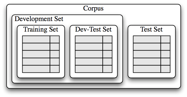
First, we select a development set, containing the corpus data for creating the model. This development set is then subdivided into the training set and the dev-test set.
train_names = labeled_names[1500:]
devtest_names = labeled_names[500:1500]
test_names = labeled_names[:500]
The training set is used to train the model and the dev-test set is used to perform error analysis. Note: it is important that we employ a separate dev-test set for error analysis rather than just using the test set. The division of the corpus data into different subsets is shown below.
We train a model using the training set [1], and then run it on the dev-test set [2]:
train_set = [(gender_features2(n), gender) for (n, gender) in train_names]
devtest_set = [(gender_features2(n), gender) for (n, gender) in devtest_names]
test_set = [(gender_features2(n), gender) for (n, gender) in test_names]
classifier = nltk.NaiveBayesClassifier.train(train_set) #[1]
print(nltk.classify.accuracy(classifier, devtest_set)) #[2]
0.739
Using the dev-test set, we can generate a list of errors that the classifier makes when predicting name genders:
errors = []
for (name, tag) in devtest_names:
    guess = classifier.classify(gender_features2(name))
    if guess != tag:
        errors.append( (tag, guess, name) )
We can then examine individual error cases where the model predicted the wrong label and try to determine what additional pieces of information would allow the classifier to make the right decision (or which existing pieces of information are tricking it into making the wrong decision). The feature set can then be adjusted accordingly.
len(errors) # number of mislabeled names
261
for (tag, guess, name) in sorted(errors):
    print('correct={:<8} guess={:<8s} name={:<30}'.format(tag, guess, name))
correct=female   guess=male     name=Agnes
correct=female   guess=male     name=Ardis
correct=female   guess=male     name=Ardys
correct=female   guess=male     name=Audy
correct=female   guess=male     name=Berte
correct=female   guess=male     name=Beth
correct=female   guess=male     name=Bo
correct=female   guess=male     name=Bobbette
correct=female   guess=male     name=Bonny
correct=female   guess=male     name=Brear
correct=female   guess=male     name=Brit
correct=female   guess=male     name=Buffy
correct=female   guess=male     name=Cam
correct=female   guess=male     name=Cameo
correct=female   guess=male     name=Carroll
correct=female   guess=male     name=Cherish
correct=female   guess=male     name=Chloris
correct=female   guess=male     name=Coriss
correct=female   guess=male     name=Correy
correct=female   guess=male     name=Cris
correct=female   guess=male     name=Cristin
correct=female   guess=male     name=Dagmar
correct=female   guess=male     name=Deborah
correct=female   guess=male     name=Doreen
correct=female   guess=male     name=Dorthy
correct=female   guess=male     name=Drew
correct=female   guess=male     name=Dulce
correct=female   guess=male     name=Easter
correct=female   guess=male     name=Elsbeth
correct=female   guess=male     name=Em
correct=female   guess=male     name=Evy
correct=female   guess=male     name=Fallon
correct=female   guess=male     name=Faythe
correct=female   guess=male     name=Florence
correct=female   guess=male     name=Francesmary
correct=female   guess=male     name=Gladys
correct=female   guess=male     name=Goldy
correct=female   guess=male     name=Gussie
correct=female   guess=male     name=Gwenore
correct=female   guess=male     name=Gwyneth
correct=female   guess=male     name=Harriott
correct=female   guess=male     name=Honor
correct=female   guess=male     name=Inez
correct=female   guess=male     name=Ingeborg
correct=female   guess=male     name=Ivett
correct=female   guess=male     name=Jerry
correct=female   guess=male     name=Jo
correct=female   guess=male     name=Joby
correct=female   guess=male     name=Joell
correct=female   guess=male     name=Joey
correct=female   guess=male     name=Josee
correct=female   guess=male     name=Joselyn
correct=female   guess=male     name=Jourdan
correct=female   guess=male     name=Karon
correct=female   guess=male     name=Kit
correct=female   guess=male     name=Korry
correct=female   guess=male     name=Kristin
correct=female   guess=male     name=Lucky
correct=female   guess=male     name=Margaret
correct=female   guess=male     name=Marget
correct=female   guess=male     name=Margo
correct=female   guess=male     name=Marjory
correct=female   guess=male     name=Marylou
correct=female   guess=male     name=Meridith
correct=female   guess=male     name=Merry
correct=female   guess=male     name=Mignon
correct=female   guess=male     name=Moll
correct=female   guess=male     name=Mommy
correct=female   guess=male     name=Myriam
correct=female   guess=male     name=Olympe
correct=female   guess=male     name=Patty
correct=female   guess=male     name=Perl
correct=female   guess=male     name=Perry
correct=female   guess=male     name=Phoebe
correct=female   guess=male     name=Phylis
correct=female   guess=male     name=Phyllis
correct=female   guess=male     name=Pru
correct=female   guess=male     name=Prudence
correct=female   guess=male     name=Rebekah
correct=female   guess=male     name=Rey
correct=female   guess=male     name=Robyn
correct=female   guess=male     name=Rosaleen
correct=female   guess=male     name=Rosalyn
correct=female   guess=male     name=Rosamond
correct=female   guess=male     name=Roselyn
correct=female   guess=male     name=Roxane
correct=female   guess=male     name=Roxie
correct=female   guess=male     name=Roxine
correct=female   guess=male     name=Rubi
correct=female   guess=male     name=Scarlet
correct=female   guess=male     name=Shanon
correct=female   guess=male     name=Sharyl
correct=female   guess=male     name=Sherry
correct=female   guess=male     name=Sheryl
correct=female   guess=male     name=Shir
correct=female   guess=male     name=Sigrid
correct=female   guess=male     name=Siobhan
correct=female   guess=male     name=Sonny
correct=female   guess=male     name=Starr
correct=female   guess=male     name=Stormi
correct=female   guess=male     name=Sue
correct=female   guess=male     name=Terese
correct=female   guess=male     name=Terry
correct=female   guess=male     name=Theo
correct=female   guess=male     name=Thomasine
correct=female   guess=male     name=Tiffy
correct=female   guess=male     name=Timmy
correct=female   guess=male     name=Tish
correct=female   guess=male     name=Torie
correct=female   guess=male     name=Torrie
correct=female   guess=male     name=Trix
correct=female   guess=male     name=Trixi
correct=female   guess=male     name=Trudey
correct=female   guess=male     name=Tuesday
correct=female   guess=male     name=Ulrike
correct=female   guess=male     name=Venus
correct=female   guess=male     name=Wandis
correct=female   guess=male     name=Wendy
correct=female   guess=male     name=Willi
correct=female   guess=male     name=Willy
correct=female   guess=male     name=Wrennie
correct=female   guess=male     name=Yoko
correct=female   guess=male     name=Zorah
correct=male     guess=female   name=Abby
correct=male     guess=female   name=Aditya
correct=male     guess=female   name=Agamemnon
correct=male     guess=female   name=Alain
correct=male     guess=female   name=Aleks
correct=male     guess=female   name=Allan
correct=male     guess=female   name=Allie
correct=male     guess=female   name=Allin
correct=male     guess=female   name=Andrea
correct=male     guess=female   name=Andri
correct=male     guess=female   name=Anthony
correct=male     guess=female   name=Antone
correct=male     guess=female   name=Antonin
correct=male     guess=female   name=Antony
correct=male     guess=female   name=Archie
correct=male     guess=female   name=Arie
correct=male     guess=female   name=Aristotle
correct=male     guess=female   name=Arne
correct=male     guess=female   name=Arvie
correct=male     guess=female   name=Arvy
correct=male     guess=female   name=Barnaby
correct=male     guess=female   name=Barny
correct=male     guess=female   name=Benjamin
correct=male     guess=female   name=Benn
correct=male     guess=female   name=Benny
correct=male     guess=female   name=Binky
correct=male     guess=female   name=Blair
correct=male     guess=female   name=Bradly
correct=male     guess=female   name=Brinkley
correct=male     guess=female   name=Cal
correct=male     guess=female   name=Chaddie
correct=male     guess=female   name=Chancey
correct=male     guess=female   name=Charlie
correct=male     guess=female   name=Chaunce
correct=male     guess=female   name=Chrissy
correct=male     guess=female   name=Clair
correct=male     guess=female   name=Clancy
correct=male     guess=female   name=Clare
correct=male     guess=female   name=Clemente
correct=male     guess=female   name=Clinton
correct=male     guess=female   name=Constantin
correct=male     guess=female   name=Cyril
correct=male     guess=female   name=Dani
correct=male     guess=female   name=Dannie
correct=male     guess=female   name=Darby
correct=male     guess=female   name=Darian
correct=male     guess=female   name=Darrin
correct=male     guess=female   name=Daryl
correct=male     guess=female   name=Dean
correct=male     guess=female   name=Deryl
correct=male     guess=female   name=Dickie
correct=male     guess=female   name=Emil
correct=male     guess=female   name=Evelyn
correct=male     guess=female   name=Ezechiel
correct=male     guess=female   name=Flynn
correct=male     guess=female   name=Gail
correct=male     guess=female   name=Galen
correct=male     guess=female   name=Garey
correct=male     guess=female   name=Gene
correct=male     guess=female   name=Gil
correct=male     guess=female   name=Glynn
correct=male     guess=female   name=Granville
correct=male     guess=female   name=Hadleigh
correct=male     guess=female   name=Hamel
correct=male     guess=female   name=Hamlen
correct=male     guess=female   name=Hanan
correct=male     guess=female   name=Hassan
correct=male     guess=female   name=Hillel
correct=male     guess=female   name=Hymie
correct=male     guess=female   name=Ike
correct=male     guess=female   name=Izzy
correct=male     guess=female   name=Jeremie
correct=male     guess=female   name=Jimmie
correct=male     guess=female   name=Jimmy
correct=male     guess=female   name=Joaquin
correct=male     guess=female   name=Jonathan
correct=male     guess=female   name=Jule
correct=male     guess=female   name=Kalvin
correct=male     guess=female   name=Keene
correct=male     guess=female   name=Kendall
correct=male     guess=female   name=Kennedy
correct=male     guess=female   name=Kin
correct=male     guess=female   name=Lane
correct=male     guess=female   name=Laurance
correct=male     guess=female   name=Lay
correct=male     guess=female   name=Lennie
correct=male     guess=female   name=Lenny
correct=male     guess=female   name=Leslie
correct=male     guess=female   name=Lindy
correct=male     guess=female   name=Linoel
correct=male     guess=female   name=Lonnie
correct=male     guess=female   name=Lovell
correct=male     guess=female   name=Luke
correct=male     guess=female   name=Lyn
correct=male     guess=female   name=Manuel
correct=male     guess=female   name=Marion
correct=male     guess=female   name=Marlin
correct=male     guess=female   name=Marlon
correct=male     guess=female   name=Martainn
correct=male     guess=female   name=Marten
correct=male     guess=female   name=Meryl
correct=male     guess=female   name=Mika
correct=male     guess=female   name=Millicent
correct=male     guess=female   name=Milt
correct=male     guess=female   name=Neal
correct=male     guess=female   name=Nealon
correct=male     guess=female   name=Nealy
correct=male     guess=female   name=Neddie
correct=male     guess=female   name=Nevil
correct=male     guess=female   name=Neville
correct=male     guess=female   name=Nilson
correct=male     guess=female   name=Noble
correct=male     guess=female   name=Obadiah
correct=male     guess=female   name=Odie
correct=male     guess=female   name=Pascale
correct=male     guess=female   name=Pierce
correct=male     guess=female   name=Rafael
correct=male     guess=female   name=Raleigh
correct=male     guess=female   name=Randall
correct=male     guess=female   name=Randell
correct=male     guess=female   name=Ray
correct=male     guess=female   name=Reggie
correct=male     guess=female   name=Rickey
correct=male     guess=female   name=Salman
correct=male     guess=female   name=Sansone
correct=male     guess=female   name=Simone
correct=male     guess=female   name=Slade
correct=male     guess=female   name=Sonnie
correct=male     guess=female   name=Stillman
correct=male     guess=female   name=Sullivan
correct=male     guess=female   name=Tait
correct=male     guess=female   name=Timmie
correct=male     guess=female   name=Virge
correct=male     guess=female   name=Yale
correct=male     guess=female   name=Yardley
correct=male     guess=female   name=Zachariah
correct=male     guess=female   name=Zacharie
correct=male     guess=female   name=Zechariah
Looking through this list of errors, it appears that certain 2-character suffixes are indicative of gender. For example, names ending in ‘yn’ appear to be predominantly female, despite the fact that names ending in ‘n’ tend to be male; and names ending in ‘ch’ are usually male, even though names that end in ‘h’ tend to be female.
Let’s adjust our feature extractor to include features for two-letter suffixes:
def gender_features(word):
    return {'suffix1': word[-1:], 'suffix2': word[-2:]}
Let’s rebuild our classifier with the new feature extractor and see whether its accuracy improves.
train_set = [(gender_features(n), gender) for (n, gender) in train_names]
devtest_set = [(gender_features(n), gender) for (n, gender) in devtest_names]
classifier = nltk.NaiveBayesClassifier.train(train_set)
print(nltk.classify.accuracy(classifier, devtest_set))
0.776
This error analysis procedure can be repeated after checking for patterns in errors made by the improved classifier. Each time the error analysis procedure is repeated, we should select a different dev-test/training split, to ensure that the classifier does not start to reflect idiosyncrasies in the dev-test set.
However, once we’ve used the dev-test set to develop the model, we can no longer trust that it will give us an accurate idea of how well the model would perform on new data. It is therefore important to keep the test set separate, and unused, until our model development is complete. At that point, we can use the test set to evaluate how well our model will perform on new input values.
Exercise
In addition to the suffix features, add another word feature to your gender classifier and evaluate the accuracy of this new model.
Document Classification
Sometimes we want to classify an entire document rather than a particular word. Document classification is especially useful for sentiment analysis because the emotions or opinions contained in a text are not typically represented by a single word.
Sentiment analysis is a category of supervised classification algorithms where the labels consist of different emotions, often negative, positive, and neutral. The procedure is the same as before: using pre-labeled corpora, we can build classifiers that automatically tag new documents with appropriate category labels.
As an illustrative example, let’s work with the Movie Reviews Corpus that categorizes each review as positive or negative.
from nltk.corpus import movie_reviews
documents = [(list(movie_reviews.words(fileid)), category)
             for category in movie_reviews.categories()
             for fileid in movie_reviews.fileids(category)]

random.shuffle(documents)
Now let’s define a feature extractor for our documents such that the classifier will know which aspects of the data it should pay attention to.
For document topic identification, we can define a feature for each word that indicates whether the document contains that word. To limit the number of features that the classifier needs to process, we begin by constructing a list of the 2000 most frequent words in the overall corpus. We can then define a feature extractor that simply checks whether each of these words is present in a given document.
all_words = nltk.FreqDist(w.lower() for w in movie_reviews.words())
word_features = list(all_words)[:2000]

def document_features(document):
    document_words = set(document)
    features = {}
    for word in word_features:
        features['contains({})'.format(word)] = (word in document_words)
    return features
Now that we’ve defined our feature extractor we can use it to train a classifier to label new movie reviews. To check how reliable the resulting classifier is, we compute its accuracy on the test set. And once again, we can use show_most_informative_features() to find out which features the classifier found to be most informative.
featuresets = [(document_features(d), c) for (d,c) in documents]
train_set, test_set = featuresets[100:], featuresets[:100]
classifier = nltk.NaiveBayesClassifier.train(train_set)
print(nltk.classify.accuracy(classifier, test_set))
0.82
classifier.show_most_informative_features(10)
Most Informative Features
 contains(unimaginative) = True              neg : pos    =      8.2 : 1.0
    contains(schumacher) = True              neg : pos    =      6.9 : 1.0
          contains(mena) = True              neg : pos    =      6.9 : 1.0
        contains(suvari) = True              neg : pos    =      6.9 : 1.0
     contains(atrocious) = True              neg : pos    =      6.5 : 1.0
        contains(shoddy) = True              neg : pos    =      6.3 : 1.0
        contains(turkey) = True              neg : pos    =      5.8 : 1.0
        contains(justin) = True              neg : pos    =      5.7 : 1.0
           contains(ugh) = True              neg : pos    =      5.7 : 1.0
       contains(unravel) = True              pos : neg    =      5.7 : 1.0
Example using Naive Bayes Classification
Let’s run some classification tasks using the Supreme Court confirmation hearings transcripts
This data contains the text of every Supreme Court confirmation hearing for which Senate Judiciary Committee transcripts are available (beginning in 1971 with hearings for Lewis Powell and William Rehnquist and concluding with Neil Gorsuch’s 2017 hearing).
import pandas as pd
import nltk

data = pd.read_csv('../input/Oct-7-2019-Supreme-Court-Confirmation-Hearing-Transcript.csv', encoding='latin1')

data = data.reset_index()

data.head()
| index | Total Order | Order | Year | Hearing | Title | Speaker (Party)(or nominated by) | Speaker and title | Statements | sentiment | |
|---|---|---|---|---|---|---|---|---|---|---|
| 0 | 0 | 1 | 1 | 2017 | Neil M. Gorsuch | Chairman | R | Senator Chuck Grassley (IA) | Chairman Grassley. Good morning, everybody. I ... | positive |
| 1 | 1 | 2 | 2 | 2017 | Neil M. Gorsuch | Nominee | R | Neil M. Gorsuch | Judge Gorsuch. Pleasure to be here. Thank you. | positive |
| 2 | 2 | 3 | 3 | 2017 | Neil M. Gorsuch | Chairman | R | Senator Chuck Grassley (IA) | Chairman Grassley. This is a big day for you a... | positive |
| 3 | 3 | 4 | 4 | 2017 | Neil M. Gorsuch | Nominee | R | Neil M. Gorsuch | Judge Gorsuch. Just a little, Senator. | neutral |
| 4 | 4 | 5 | 5 | 2017 | Neil M. Gorsuch | Chairman | R | Senator Chuck Grassley (IA) | Chairman Grassley. Yes. Before we begin, I wou... | neutral |
Classifying partisanship
Do Republicans and Democrats speak differently at judicial confirmation hearings? That is, can we infer party label based on what a speaker says?
The dataset already includes the party label of each speaker. We can use this information to create a partisanship classifier.
The first thing we need to do to create our classifier is to create a set of word features associated with a given party label. There are a few pre-processing steps we will need to do in order to extract the labeled text features from our pandas dataframe object so it can be added to our classifier.
Pre-processing steps
The first thing we want to do is create a list of all words across all documents. Recall that this information is used to calculate the posterior probabilities in naive bayes classification.
Let’s begin by tokenizing all of the documents.
words = data['Statements'].apply(nltk.word_tokenize)
words # the tokenized words are structured as a dataframe.
0        [Chairman, Grassley, ., Good, morning, ,, ever...
1        [Judge, Gorsuch, ., Pleasure, to, be, here, .,...
2        [Chairman, Grassley, ., This, is, a, big, day,...
3        [Judge, Gorsuch, ., Just, a, little, ,, Senato...
4        [Chairman, Grassley, ., Yes, ., Before, we, be...
                               ...
30173    [Mr., POWELL, ., I, wish, to, thank, the, chai...
30174    [The, CHAIRMAN, ., Thank, you, ,, sir, ., Now,...
30175    [Senator, SCOTT, ., IS, that, room, 2300, ,, M...
30176    [The, CHAIRMAN, ., It, is, the, Judiciary, Com...
30177    [Senator, SCOTT, ., Room, 2228, ., I, just, sa...
Name: Statements, Length: 30178, dtype: object
Turn this dataframe into a list object.
words = list(words) # the tokenized words are now structured as a list of lists
Create a master list of all words ** across **all documents. This list will be used to construct our features set below.
import itertools
all_words = (list(itertools.chain.from_iterable(words))) # we will use this information below when we build our naive bayes classifier.
Now let’s pre-process the text in the original dataframe, tokenizing words and converting everything to lower case.
data['Statements'] = data['Statements'].apply(lambda x: x.lower())
data['Statements'] = data['Statements'].apply(nltk.word_tokenize)
Create a list object that links texts with party label. We will split this data up into a training and test set for our classifier.
documents = list(zip(data['Statements'], data['Speaker (Party)(or nominated by)']))
Now let’s use this information to create a features extractor for our documents. The following features extractor indicates whether a given document contains a word from our master lists of words (all_words). To limit the number of features that the classifier needs to process, we begin by constructing a list of the 2000 most frequent words in the overall corpus [1]. We then define a feature extractor [2] that simply checks whether each of these words is present in a given document.
all_words = nltk.FreqDist(w.lower() for w in all_words) #[1]
word_features = list(all_words)[:2000]

def document_features(document): #[2]
    document_words = set(document)
    features = {}
    for word in word_features:
        features['contains({})'.format(word)] = (word in document_words)
    return features
Now that we’ve defined our feature extractor, we can use it to train a classifier to label new, previously unseen texts. To check how reliable the resulting classifier is, we compute its accuracy on the test set. And once again, we can use the command show_most_informative_features( ) to find out which features the classifier found to be most informative.
featuresets = [(document_features(d), c) for (d,c) in documents]
train_set, test_set = featuresets[100:], featuresets[:100]
classifier = nltk.NaiveBayesClassifier.train(train_set)
classifier.show_most_informative_features(5)
Most Informative Features
       contains(kennedy) = True                D : nan    =     37.5 : 1.0
   contains(innumerable) = True              nan : R      =     26.6 : 1.0
       contains(gorsuch) = True                R : D      =     26.4 : 1.0
     contains(important) = True                R : nan    =     25.6 : 1.0
         contains(judge) = True                R : nan    =     25.5 : 1.0
print(nltk.classify.accuracy(classifier, test_set))
0.35
With approximately 35% accuracy, this is a pretty abysmal classifier. This classifier performs more poorly than if we just flipped a coin to assign party label (i.e. 50% accuracy)!
What could we do to improve our classifier? How about we restrict our sample to a single confirmation hearing, i.e. Neil Gorsuch’s hearing in 2017? How well does the classifier perform for this subset?
data = pd.read_csv('../input/Oct-7-2019-Supreme-Court-Confirmation-Hearing-Transcript.csv', encoding='latin1')
data = data.reset_index()


data = data[data['Statements'].notnull() & (data['Year'] == 2017)] # only hearings from 2017
words = data['Statements'].apply(nltk.word_tokenize)
words = list(words)

all_words = (list(itertools.chain.from_iterable(words)))


data['Statements'] = data['Statements'].apply(lambda x: x.lower())
data['Statements'] = data['Statements'].apply(nltk.word_tokenize)


documents = list(zip(data['Statements'], data['Speaker (Party)(or nominated by)']))

all_words = nltk.FreqDist(w.lower() for w in all_words)
word_features = list(all_words)[:2000]

def document_features(document):
    document_words = set(document)
    features = {}
    for word in word_features:
        features['contains({})'.format(word)] = (word in document_words)
    return features

featuresets = [(document_features(d), c) for (d,c) in documents]
train_set, test_set = featuresets[100:], featuresets[:100]
classifier = nltk.NaiveBayesClassifier.train(train_set)

print(nltk.classify.accuracy(classifier, test_set))
0.87
Restricting our classifier to 2017 improved our accuracy by over 50%! Why do you think the classifier does a better job on 2017 than for the corpus as a whole?
Exercises
- Using the sentiment labels you constructed for the Supreme Court Confirmation Hearings transcripts, use a Naive Bayes classifier to predict the sentiment of statements made by and before the Senate Judiciary Committee.
- Evaluate the accuracy of your classifier.
- Run error analysis on your classifier. Which features are contributing to misclassification?
- Try improving the accuracy of your classifier by adding or substracting word features or subsetting the data.